Contrasts against Control: Dunnet vs. Holm vs. TukeyHSD
TLDR: Even though Dunnet is proven to be optimal (in all vs comparison) for a reasonable group number (around 10) Holm seems to yield basically the same result, while being a more general method. Dunnet is more powerful, when increasing the group number (e.g., to 30).
Purpose and Structure of this Document
In many cases, we may want to compare new alternatives to a standard treatment or control. To do this, we use a linear model and perform hypothesis testing of all alternatives versus the control. The purpose of this document is to compare the power of different multiple testing techniques.
The document is structured as follows:
- Define helper functions, including:
- data generation
- multiple testing functions
- wrapper for simulations
- Perform simulations for various settings.
- Plot the results.
Note, that there are different definitions of “power” in this context. We will be using the following definitions:
- The expectation that any of the non-placebos will be rejected.
- The expectation of the fraction of non-placebos that will be rejected.
- The expectation that all non-placebos will be rejected.
Help functions
set.seed(123)
n_rep <- 1000

library(multcomp)
library(PMCMRplus)
library(ggplot2)

# g groups, of which one is the control, n_effect of which have the effect `effect`
get_data <- function(g = 10, n_t = 5, n_c = 5, effect = 1, n_effect = 3) {
  fac <- as.factor(
    rep(c("ctrl", c(LETTERS, letters)[1:(g - 1)]),
    c(n_c, rep(n_t, g - 1)))
    )
  groups <- relevel(fac, ref = "ctrl")
  y <- rnorm(groups,
    c(rep(0, length(groups) - n_t * n_effect), rep(effect, n_t * n_effect))
    )
  data.frame(group = groups, y = y)
}

holm <- function(data) {
  fit <- lm(y ~ group, data)
  p_vals <- summary(fit)$coefficients[-1, "Pr(>|t|)"]
  p.adjust(p_vals)
}

none <- function(data) {
  fit <- lm(y ~ group, data)
  summary(fit)$coefficients[-1, "Pr(>|t|)"]
}

tukey_hsd <- function(data) {
  fit <- aov(y ~ group, data)
  a <- TukeyHSD(fit)
  contrasts <- grep("ctrl", rownames(a$group), value = TRUE)
  a$group[contrasts, "p adj"]
}

# multcomp implementation of "dunnet"
dunn <- function(data) {
  n <- table(data$group)
  names(n) <- levels(data$group)
  c(summary(
    glht(aov(y ~ group, data), linfct = mcp(group = "Dunnett"))
  )$test$pvalues)
}

all <- function(data) as.matrix(data.frame(none = none(data),
  holm = holm(data), dunn = dunn(data), tukeyHSD = tukey_hsd(data))
)

dosim <- function(n_replicate = 200, n_goups = 10, n_treatmentgroup = 5,
                  n_controlgroup = 5, effect = 1, n_non_placebo_treatments = 3) {
  obj <- mcreplicate::mc_replicate(n_replicate, all(get_data(
    g = n_goups, n_t = n_treatmentgroup, n_c = n_controlgroup, effect = effect,
    n_effect = n_non_placebo_treatments
  )))
  stopifnot(effect > 0)
  if (n_non_placebo_treatments == 0) {
    p_val_non_placebo <- obj
    p_val_non_placebo[, , ] <- 1 # this is used for power calc. In this case no effect
  } else {
    p_val_non_placebo <- obj[(n_goups - n_non_placebo_treatments):(n_goups - 1), , ]
  }
  p_val_no_effect <- obj[1:(n_goups - n_non_placebo_treatments - 1), , ]

  # The fraction of rejected tests within the non-placebo treatments
  MeanPower <- apply(p_val_non_placebo, 2, function(x) mean(x < 0.05))
  names(MeanPower) <- paste0("MeanPower_", names(MeanPower))

  # The fraction where all non-placebo treatments where detected
  AllPower  <- apply(p_val_non_placebo, c(2, 3), function(x) base::all(x < 0.05))
  AllPower  <- apply(AllPower, 1, function(x) mean(x))
  names(AllPower) <- paste0("AllPower_", names(AllPower))

  # The fraction where ANY non-placebo treatment was detected
  AnyPower  <- apply(p_val_non_placebo, c(2, 3), function(x) base::any(x < 0.05))
  AnyPower  <- apply(AnyPower, 1, function(x) mean(x))
  names(AnyPower) <- paste0("AnyPower_", names(AnyPower))

  # The FWER under the NULL (i.e. for placebo treatments)
  any_positive <- apply(p_val_no_effect, c(2, 3), function(x) any(x < 0.05))
  alpha <- apply(any_positive, 1, function(x) mean(x))
  names(alpha) <- paste0("alpha_", names(alpha))

  as.matrix(c(
    n_replicate = n_replicate, n_goups = n_goups,
    n_treatmentgroup = n_treatmentgroup,
    n_controlgroup = n_controlgroup, effect = effect,
    n_non_placebo_treatments = n_non_placebo_treatments,
    MeanPower, AllPower, AnyPower, alpha
  ), ncol = 1)
}
Simulations
a <- dosim(n_replicate = n_rep, n_non_placebo_treatments = 0) # NULL
g <- dosim(n_replicate = n_rep)
b <- dosim(n_replicate = n_rep, effect = .5)
c <- dosim(n_replicate = n_rep, effect = 2)
# 12=floor(n_t * sqrt(g-1)) ==> taking 14 yields the same total sample size
d <- dosim(n_replicate = n_rep, n_treatmentgroup = 4, n_controlgroup = 14)
e <- dosim(n_replicate = n_rep, n_treatmentgroup = 4, n_controlgroup = 14, effect = 2)
f <- dosim(n_replicate = n_rep, n_treatmentgroup = 4, n_controlgroup = 14,
            n_non_placebo_treatments = 7)
h <- dosim(n_replicate = n_rep, n_goups = 30, n_non_placebo_treatments = 3)
i <- dosim(n_replicate = n_rep, n_goups = 30, n_non_placebo_treatments = 10)
j <- dosim(n_replicate = n_rep, n_goups = 30, n_non_placebo_treatments = 20)
k <- dosim(n_replicate = n_rep, n_treatmentgroup = 20, n_controlgroup = 20)
# optimal sample allocation with equal total
l <- dosim(n_replicate = n_rep, n_treatmentgroup = 17, n_controlgroup = 47)
Results
result <- cbind(
  null=a,
  default=g,
  `-effect`=b,
  `+effect`=c,
  `+alloc` = d,
  `+alloc+effect` = e,
  `+nonplacebo_grps`=f,
  `+grps`=h,
  `+grps+nonplacebo`=i,
  `+grps++nonplacebo`=j,
  `+groupsize`=k,
  `+grpsize+alloc`=l
)
colnames(result) <- c("null", "default", "`-effect`", "`+effect`", "`+alloc`",
  "`+alloc+effect`", "`+nonplacebo_grps`", "`+grps`", "`+grps+nonplacebo`",
  "`+grps++nonplacebo`", "`+groupsize`", "`+grpsize+alloc`"
)
options(digits=4)
result |> as.data.frame() |> knitr::kable()
| null | default | -effect |
+effect |
+alloc |
+alloc+effect |
+nonplacebo_grps |
+grps |
+grps+nonplacebo |
+grps++nonplacebo |
+groupsize |
+grpsize+alloc |
|
|---|---|---|---|---|---|---|---|---|---|---|---|---|
| n_replicate | 1000.000 | 1000.0000 | 1000.0000 | 1000.0000 | 1000.0000 | 1000.0000 | 1000.0000 | 1000.0000 | 1000.0000 | 1000.0000 | 1000.0000 | 1000.0000 |
| n_goups | 10.000 | 10.0000 | 10.0000 | 10.0000 | 10.0000 | 10.0000 | 10.0000 | 30.0000 | 30.0000 | 30.0000 | 10.0000 | 10.0000 |
| n_treatmentgroup | 5.000 | 5.0000 | 5.0000 | 5.0000 | 4.0000 | 4.0000 | 4.0000 | 5.0000 | 5.0000 | 5.0000 | 20.0000 | 17.0000 |
| n_controlgroup | 5.000 | 5.0000 | 5.0000 | 5.0000 | 14.0000 | 14.0000 | 14.0000 | 5.0000 | 5.0000 | 5.0000 | 20.0000 | 47.0000 |
| effect | 1.000 | 1.0000 | 0.5000 | 2.0000 | 1.0000 | 2.0000 | 1.0000 | 1.0000 | 1.0000 | 1.0000 | 1.0000 | 1.0000 |
| n_non_placebo_treatments | 0.000 | 3.0000 | 3.0000 | 3.0000 | 3.0000 | 3.0000 | 7.0000 | 3.0000 | 10.0000 | 20.0000 | 3.0000 | 3.0000 |
| MeanPower_none | 0.000 | 0.3410 | 0.1113 | 0.8683 | 0.4030 | 0.9343 | 0.3891 | 0.3467 | 0.3603 | 0.3532 | 0.8890 | 0.9377 |
| MeanPower_holm | 0.000 | 0.1130 | 0.0203 | 0.6123 | 0.1427 | 0.7437 | 0.1440 | 0.0587 | 0.0702 | 0.0646 | 0.6650 | 0.7853 |
| MeanPower_dunn | 0.000 | 0.1283 | 0.0257 | 0.6407 | 0.1453 | 0.7317 | 0.1393 | 0.0787 | 0.0847 | 0.0762 | 0.6837 | 0.7777 |
| MeanPower_tukeyHSD | 0.000 | 0.0547 | 0.0060 | 0.4413 | 0.0703 | 0.5607 | 0.0654 | 0.0150 | 0.0185 | 0.0146 | 0.4850 | 0.6343 |
| AllPower_none | 0.000 | 0.1420 | 0.0190 | 0.7240 | 0.1220 | 0.8240 | 0.0140 | 0.1290 | 0.0480 | 0.0150 | 0.7520 | 0.8430 |
| AllPower_holm | 0.000 | 0.0240 | 0.0010 | 0.3900 | 0.0160 | 0.4800 | 0.0010 | 0.0090 | 0.0000 | 0.0010 | 0.4430 | 0.5530 |
| AllPower_dunn | 0.000 | 0.0250 | 0.0010 | 0.4050 | 0.0140 | 0.4430 | 0.0010 | 0.0150 | 0.0000 | 0.0000 | 0.4480 | 0.5310 |
| AllPower_tukeyHSD | 0.000 | 0.0050 | 0.0000 | 0.2140 | 0.0030 | 0.2640 | 0.0000 | 0.0020 | 0.0000 | 0.0000 | 0.2520 | 0.3400 |
| AnyPower_none | 0.000 | 0.5640 | 0.2410 | 0.9740 | 0.7060 | 0.9990 | 0.9010 | 0.5830 | 0.8090 | 0.8910 | 0.9820 | 0.9960 |
| AnyPower_holm | 0.000 | 0.2270 | 0.0480 | 0.8210 | 0.3300 | 0.9470 | 0.4970 | 0.1320 | 0.2810 | 0.3540 | 0.8620 | 0.9630 |
| AnyPower_dunn | 0.000 | 0.2650 | 0.0620 | 0.8550 | 0.3420 | 0.9520 | 0.5160 | 0.1730 | 0.3350 | 0.4210 | 0.8920 | 0.9680 |
| AnyPower_tukeyHSD | 0.000 | 0.1250 | 0.0160 | 0.6840 | 0.1830 | 0.8440 | 0.2970 | 0.0370 | 0.1100 | 0.1410 | 0.7300 | 0.9080 |
| alpha_none | 0.277 | 0.1860 | 0.1980 | 0.1960 | 0.2410 | 0.2530 | 0.0890 | 0.4260 | 0.4340 | 0.3030 | 0.1900 | 0.2280 |
| alpha_holm | 0.035 | 0.0310 | 0.0170 | 0.0290 | 0.0290 | 0.0430 | 0.0130 | 0.0330 | 0.0300 | 0.0140 | 0.0330 | 0.0290 |
| alpha_dunn | 0.048 | 0.0370 | 0.0230 | 0.0290 | 0.0300 | 0.0370 | 0.0110 | 0.0530 | 0.0490 | 0.0180 | 0.0350 | 0.0250 |
| alpha_tukeyHSD | 0.010 | 0.0110 | 0.0040 | 0.0070 | 0.0090 | 0.0100 | 0.0030 | 0.0080 | 0.0040 | 0.0000 | 0.0030 | 0.0040 |
Plot
X <- result[-c(1:7, 11, 15, 19),] # remove "none" rows, and parameters

# convert matrix to data frame
df <- data.frame(env = rep(colnames(X), each = nrow(X)),
                 strategy = rep(rownames(X), times = ncol(X)),
                 value = as.vector(X))

# split the strategy names into two parts
df$part1 <- gsub("^(.*?)_.*$", "\\1", df$strategy)
df$part2 <- gsub("^.*?_(.*)$", "\\1", df$strategy)

# plot
plt <- ggplot(df, aes(x = factor(env, ordered=T, levels=unique(env)), y = value,
  group = strategy, linetype = part1, color = part2)) +
  geom_line() +
  geom_point() +
  scale_linetype_manual(
    values = c("solid", "dashed", "dotted", "dotdash")) +  # line types
  theme(axis.text.x = element_text(angle = 30, hjust = 1)) # vertical x-labels
plt
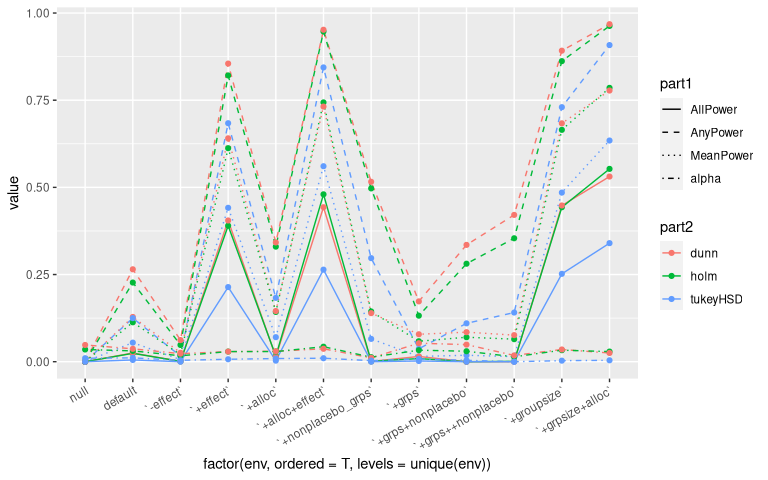
Results
- Dunnet and Holm yield very similar results when considering 10 groups (while varying the number of non-placebo groups, the effect, and the sample size allocation).
- Dunnet shows a slight advantage over Holm, when increasing the number of groups.
- The optimal allocation ($n_{control} = n_{treatments}\sqrt{n_{groups}-1}$) yields an improvement as well in both cases.