Testing Slopes in a LMM – Should we Simplify?
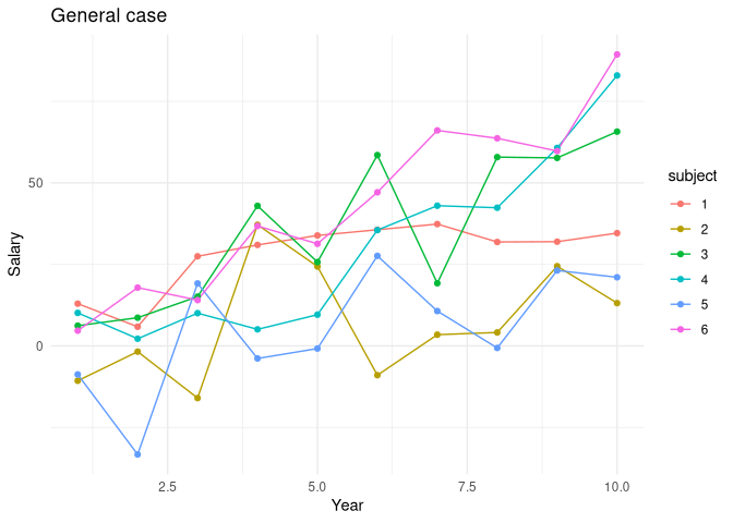
TLDR: Given a dataset as shown in the last plot, we consider the following analyses:
- For each subject extract the slope and perform a simple t-test on the slopes
- Fit
lmer(salery ~ slope + (1|subject))and test if $\beta_{slope} =0$ - Fit
lmer(salery ~ slope + (slope|subject))and test if $\beta_{slope} =0$
Then: 1 & 3 are valid (if data balanced, they are equally powerful) approaches and 2 is only valid if there is no individual slope.
Simulate Data
Salary of subject $s$ at time $t$:
\[salary_{t}^{(s)} = t \cdot (slope + d_s) + intercept_s + \varepsilon_{t,s}\]- $d_s \sim \mathcal N(0, subjSlopeSD^2)$
- $intercept_s \sim \mathcal N(0, subjSD^2)$
- $\varepsilon_{t,s} \sim \mathcal N(0, obsSD^2)$
nsim <- 2000

library(mcreplicate) # for parallelization
library(ggplot2)
library(lmerTest)

#' `nsub`: how many subjects (default: 6)
#' `nyears`: how many years(default: 10)
#' `obsSD`: standard deviation of noise (observation-level) (default: 15)
#' `subjSD`: standard deviation of individual effect (default: 4)
#' `slope`: shared increase of income per year (default: 5)
#' `subjSlopeSD`: subject specific standard deviation from slope (default: 2)
get_data <- function(nsub=6, nyears=10,
                     obsSD=15, subjSD=4,
                     slope=5, subjSlopeSD=2){
  subj_intercept <- rep(rnorm(nsub, 0, subjSD), each=nyears)
  subj_slope <- rep(rnorm(nsub, slope, subjSlopeSD), each=nyears)
  data.frame(
    subject = as.factor(rep(1:nsub, each = nyears)),
    year = rep(1:nyears, times = nsub),
    salary =  subj_intercept +  # subject effect
              subj_slope*(1:nyears) + # individual slope
              rnorm(nyears*nsub, 0, obsSD) # obsSD
  )
}
Plot Data
plot_data <- function(main, ...){
  ggplot(get_data(...), aes(x = year, y = salary, group = subject, color = subject)) +
    geom_line() +
    geom_point() +
    labs(x = "Year", y = "Salary") +
    theme_minimal() +
    ggtitle(main)
}
set.seed(123)
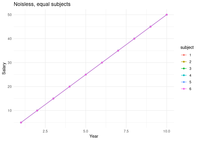
plot_data("Noisless, equal subjects", obsSD=0, subjSD=0, subjSlopeSD=0)
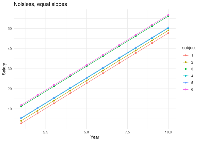
plot_data("Noisless, equal slopes", obsSD=0, subjSlopeSD=0)
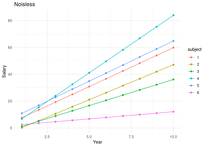
plot_data("Noisless", obsSD=0)
plot_data("General case")
Analysis Methods
slopeTTest <- function(data){
  fits <- lmList(salary ~ year | subject, data)
  slopes <- coef(fits)[,"year"]
  t_test <- t.test(slopes, mu = 0)
  t_test$p.value
}

lmmRandItcpt <- function(data){
  lmm <- lmer(salary ~ year + (1|subject), data = data)
    summary(lmm)$coefficients[2, "Pr(>|t|)"]
}

lmmRandSlope <- function(data){
  lmm <- lmer(salary ~ year + (year|subject), data = data)
    summary(lmm)$coefficients[2, "Pr(>|t|)"]
}

p_values <- function(...){
  data <- get_data(...)
  c(
    slopeTTest = slopeTTest(data),
    lmmRandItcpt = lmmRandItcpt(data),
    lmmRandSlope = lmmRandSlope(data)
  ) # if you cange the amount of arguments, change also the object "Power"
}

get_power <- function(...){
  args <- list(...)
  PVALS <- as.data.frame(t(
  mc_replicate(nsim, do.call(p_values, args))
  ))
  # POWER:
  sapply(lapply(PVALS, function(x) x<0.05), mean)
}
Power Calculations
set.seed(123)
ARGS <- as.data.frame(rbind(
  # NULL:
  expand.grid(
    nsub=6,
    nyears=10,
    obsSD=5,
    subjSD=4,
    slope=0,
    subjSlopeSD=c(0,4)),
  # Change standard deviations and effects:
  expand.grid(
    nsub=6,
    nyears=10,
    obsSD=c(5,15),
    subjSD=c(4, 12),
    slope=c(2,4),
    subjSlopeSD=c(1,4)),
  # Change samplesize (allocation):
  expand.grid(
    nsub=c(6,10,20),
    nyears=c(10,20),
    obsSD=5,
    subjSD=4,
    slope=2,
    subjSlopeSD=1)[-1,]
))
rownames(ARGS) <- NULL

Power <- matrix(NA, nrow=nrow(ARGS), ncol=3)
colnames(Power) <- c("slopeTTest",
  "lmmRandItcpt", "lmmRandSlope")

for (i in 1:nrow(ARGS)){
  args <- as.list(ARGS[i,])
  Power[i,] <- do.call(get_power, args)
}
Show Results:
as.data.frame(cbind(ARGS, Power)) |> knitr::kable()
| nsub | nyears | obsSD | subjSD | slope | subjSlopeSD | slopeTTest | lmmRandItcpt | lmmRandSlope |
|---|---|---|---|---|---|---|---|---|
| 6 | 10 | 5 | 4 | 0 | 0 | 0.0500 | 0.0510 | 0.0235 |
| 6 | 10 | 5 | 4 | 0 | 4 | 0.0475 | 0.5100 | 0.0475 |
| 6 | 10 | 5 | 4 | 2 | 1 | 0.9230 | 0.9995 | 0.9210 |
| 6 | 10 | 15 | 4 | 2 | 1 | 0.5580 | 0.8065 | 0.5255 |
| 6 | 10 | 5 | 12 | 2 | 1 | 0.9315 | 1.0000 | 0.9315 |
| 6 | 10 | 15 | 12 | 2 | 1 | 0.5335 | 0.7925 | 0.5155 |
| 6 | 10 | 5 | 4 | 4 | 1 | 1.0000 | 1.0000 | 1.0000 |
| 6 | 10 | 15 | 4 | 4 | 1 | 0.9760 | 0.9985 | 0.9760 |
| 6 | 10 | 5 | 12 | 4 | 1 | 1.0000 | 1.0000 | 1.0000 |
| 6 | 10 | 15 | 12 | 4 | 1 | 0.9755 | 1.0000 | 0.9755 |
| 6 | 10 | 5 | 4 | 2 | 4 | 0.1670 | 0.7395 | 0.1680 |
| 6 | 10 | 15 | 4 | 2 | 4 | 0.1340 | 0.6015 | 0.1280 |
| 6 | 10 | 5 | 12 | 2 | 4 | 0.1730 | 0.7240 | 0.1730 |
| 6 | 10 | 15 | 12 | 2 | 4 | 0.1555 | 0.5830 | 0.1520 |
| 6 | 10 | 5 | 4 | 4 | 4 | 0.5100 | 0.9655 | 0.5100 |
| 6 | 10 | 15 | 4 | 4 | 4 | 0.4550 | 0.9000 | 0.4465 |
| 6 | 10 | 5 | 12 | 4 | 4 | 0.5115 | 0.9645 | 0.5110 |
| 6 | 10 | 15 | 12 | 4 | 4 | 0.4395 | 0.9175 | 0.4355 |
| 10 | 10 | 5 | 4 | 2 | 1 | 0.9970 | 1.0000 | 0.9970 |
| 20 | 10 | 5 | 4 | 2 | 1 | 1.0000 | 1.0000 | 1.0000 |
| 6 | 20 | 5 | 4 | 2 | 1 | 0.9615 | 1.0000 | 0.9615 |
| 10 | 20 | 5 | 4 | 2 | 1 | 0.9990 | 1.0000 | 0.9990 |
| 20 | 20 | 5 | 4 | 2 | 1 | 1.0000 | 1.0000 | 1.0000 |