Does the variance of the Random-Effect influence the p-values?
We study the classical setup of a randomized complete block design with 2 treatments, 2 replications per block and 5 blocks. We vary the variance of the block effect and study how the p-values of the treatment effect change.
\[% equatiomatic::extract_eq(fit) \begin{aligned} \operatorname{y}_{i} &\sim N \left(\alpha_{block(i)} + \beta_{trt(i)}, \sigma^2 \right) \\ \alpha_{j} &\sim N \left(\mu_{\alpha_{j}}, {\sigma_{\alpha_{j}}}^2 \right) \text{, for block j = 1,} \dots \text{,5}\\ % contr sum for \beta_{trt(i)}: \beta_{1} &= - \beta_{2} \quad \text{(contr.sum)} \end{aligned}\]TLDR
The p-values of the treatment effect are not influenced by the variance of the block effect in our example.
Simulate Data
library(ggplot2)
library(lmerTest)

options(contrasts = c("contr.sum", "contr.poly"))
# simulate data for a linear mixed model
# a randomized complete block design with 3 treatments, nblock blocks, nrep replicates per block
# an observation error with standard deviation SD_noise and a block effect with standard deviation SD_block
# a treatment effect with standard deviation SD_trt
get_data <- function(nblock=5, nrep=2, SD_noise=3, SD_block=1, SD_trt=0) {
  data <- expand.grid(
    nrep = 1:nrep,
    trt = as.factor(1:2),
    block = as.factor(1:nblock)
  )
  block_effect <- SD_block * rnorm(nblock)[data$block]
  noise <- SD_noise * rnorm(nrow(data))
  trt_effect <- SD_trt * rnorm(nrow(data))[data$trt]
  data$y <- trt_effect + block_effect + noise
  data
}
Plot Function
# function that makes an interactions plot
plot_interactions <- function(data, ...) {
  with(data,
  interaction.plot(
      x.factor = trt,
      trace.factor = block,
      response = y,
      type = "b",
      legend = FALSE,
      ...
    )
  )
}
Perform Analysis
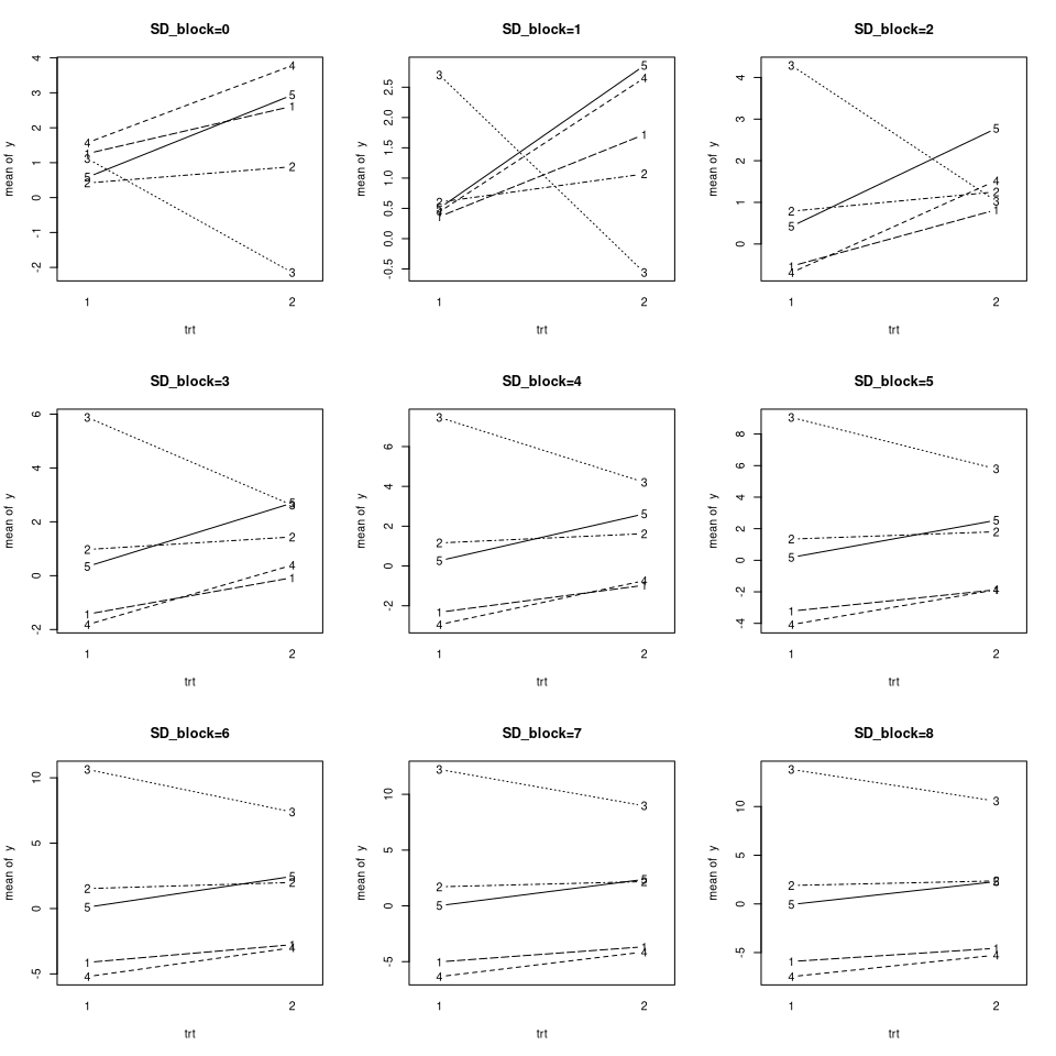
- Get Data that only differs with respect to SD_block (increasing)
- Plot the data for each SD_block
- Fit a model with lmer and lm for each SD_block
- inspect how the estimates and standard errors of the treatmenteffect change with increasing SD_block
SD_blocks <- 0:8
fits <- vector("list", length(SD_blocks)*2)
dim(fits) <- c(length(SD_blocks), 2)
dimnames(fits) <- list(paste0("SD_block=",as.character(SD_blocks)), c("lmer", "lm"))

par(mfrow=c(3,3))
for(i in seq_along(SD_blocks)){
  SD_block <- SD_blocks[i]

  set.seed(2)
  data <- get_data(SD_block=SD_block)
  plot_interactions(data, main=paste0("SD_block=", SD_block))

  # lmer
  fits[[i,1]] <- lmer(y ~ trt + (1|block), data=data)

  # lm
  fits[[i,2]] <- lm(y ~ trt + block, data=data)
}; par(mfrow=c(1,1))
boundary (singular) fit: see help('isSingular')
boundary (singular) fit: see help('isSingular')
boundary (singular) fit: see help('isSingular')
# apply a function to each element of a list-array
# preserving the dimensions and dimnames
elementwise_apply <- function(L, f){
  L_applied <- lapply(L, f)
  dim(L_applied) <- dim(L)
  dimnames(L_applied) <- dimnames(L)
  L_applied
}

summary_coef_trt1 <- elementwise_apply(fits, function(fit) coef(summary(fit))["trt1",])
Results
Illustration: How summary_coef_trt1 looks like:
summary_coef_trt1["SD_block=5",]
$lmer
  Estimate Std. Error         df    t value   Pr(>|t|)
  -0.31258    0.85616   14.00000   -0.36510    0.72049

$lm
  Estimate Std. Error    t value   Pr(>|t|)
  -0.31258    0.85616   -0.36510    0.72049
# estimate
elementwise_apply(summary_coef_trt1, function(coef) coef[1])
           lmer     lm
SD_block=0 -0.31258 -0.31258
SD_block=1 -0.31258 -0.31258
SD_block=2 -0.31258 -0.31258
SD_block=3 -0.31258 -0.31258
SD_block=4 -0.31258 -0.31258
SD_block=5 -0.31258 -0.31258
SD_block=6 -0.31258 -0.31258
SD_block=7 -0.31258 -0.31258
SD_block=8 -0.31258 -0.31258
# standard error
elementwise_apply(summary_coef_trt1, function(coef) coef[2])
           lmer    lm
SD_block=0 0.79971 0.85616
SD_block=1 0.75889 0.85616
SD_block=2 0.78422 0.85616
SD_block=3 0.85616 0.85616
SD_block=4 0.85616 0.85616
SD_block=5 0.85616 0.85616
SD_block=6 0.85616 0.85616
SD_block=7 0.85616 0.85616
SD_block=8 0.85616 0.85616
# p-value
elementwise_apply(summary_coef_trt1, function(coef) coef[length(coef)])
           lmer    lm
SD_block=0 0.70048 0.72049
SD_block=1 0.68528 0.72049
SD_block=2 0.69488 0.72049
SD_block=3 0.72049 0.72049
SD_block=4 0.72049 0.72049
SD_block=5 0.72049 0.72049
SD_block=6 0.72049 0.72049
SD_block=7 0.72049 0.72049
SD_block=8 0.72049 0.72049
# random effect variance
sapply(fits[,1], function(fit) VarCorr(fit)$block[1]) |> sqrt() |> signif(2)
SD_block=0 SD_block=1 SD_block=2 SD_block=3 SD_block=4 SD_block=5 SD_block=6
      0.00       0.00       0.00       0.73       2.50       3.70       4.90
SD_block=7 SD_block=8
      6.00       7.20